Integrated approach vs. two-step approaches • PIPScreening

library(PIPScreening)

Scenario setting

True physical model is \[\zeta_i(x_1,x_2)=x_1+x_2,.\]

The field data are for \(i=1,\ldots,N\) : \[y_i=\zeta(\mathbf{x_i})+\epsilon_i\,.\]

where \(\epsilon_i\overset{iid}{\sim}\mathcal{N}(0,\sigma^2_\epsilon)\).

Our computer model / simulator is \[f(\mathbf{x},{\theta})= \theta x_1+(1-\theta)x_2\,.\] The parameter \({\theta}\) is a model parameter, it may be fixed or be to calibrate. This parameter tunes which of the input variables \(x_1\) or \(x_2\) is taken into account with the constraint that they cannot be both active.

Data simulation

Field data:

set.seed(123)
N<-50
theta<-.5 # choice of the theta (here same size as x)
sd<-0.05
scalefactor = 10
# x1 <- seq(0,1,length.out=N)
# x2 <- seq(0,1,length.out=N)
x1 <- runif(N,0,1)
x2 =  runif(N,0,1)
simGal <- function(x){(x[,1]+x[,2])*scalefactor} 
x <- cbind(x1,x2)
mu <- simGal(x) # physical system
y <- mu + rnorm(N,0,sd) # field exp by adding noise

Preparing the data for running the MCMC run:

simulator = function(x,theta){(c(theta)*x[,1]+c(1-theta)*x[,2])*scalefactor}# computer model (if we multiply the output of the model by 2 we recover the true physical system for theta=.5)
mod <- simulator(x, .5) # output of computer model
xnorm <- (x - matrix(apply(x,2,min),nrow=nrow(x),ncol=ncol(x),byrow=T))/matrix(apply(x,2,max)-apply(x,2,min),nrow=nrow(x),ncol=ncol(x),byrow=T) # normalization
Yexp <- y; Xexpnorm <- xnorm; Xexp <- x;  Rexp <- (y-mod)

Posterior sampling with or without calibration

Without calibration (\(\boldsymbol{\theta}\) being fixed to 0.5 which is a nominal value)

calibration1 <- list(computermodel=simulator,Yexp=Yexp,Xexp=Xexp,FALSE)
tdistFULL <- tensordist(xnorm)
pgamma <-  2
parwalk = c(rep(.1,pgamma),.1,.1)*5
parwalkinit  <-  parwalk
init  <-  c(rep(0,pgamma),.004,.2)
parprior <- rbind(matrix(1,nrow=pgamma,ncol=2),c(4,.02),c(3,1))
nMWG <- 5000
nMet <- 10000
resmcmc <- (MCMC(nMWG,nMet,parwalkinit,init,Rexp,tdistFULL,1.9,parprior,TRUE,calibration1))

With calibration, we just changed some options to run this version such as the calibration2 list which indicates that calibration should be done, the init2 vector which gives the initial value for all the parameters (now it includes the \(\theta\)s) and the parwalkinit2 which gives the parameter for the random walk.

ptheta <- 1
calibration2 <- list(computermodel=simulator,Yexp=Yexp,Xexp=Xexp,TRUE)
parwalkinit2 <- c(parwalk,rep(.5,ptheta))
init2 <- c(rep(0,pgamma),.004,.2,rep(.5,ptheta))
resmcmccal <- MCMC(nMWG,nMet,parwalkinit2,init2,Rexp,tdistFULL,1.9,parprior,TRUE,calibration2)

The sampling is done with a Metropolis within Gibbs algorithm and then with a Metropolis algorithm. From the MwG algorithm, a covariance matrix is derived for the random walk in the upcoming Metropolis algorithm. Some adaptations are performed to set the exploration step. Note the number of iterations are really low in this vignette to limit its compilation time.

Computation of probabilites of activeness

First computed from the posterior sampling without calibration and then computed from the posterior sampling which deals with calibration. We obtain then two vectors of probabilities which give for each variable the probability that a variable is active in the discrepancy. Here we expect that both variables may be active.

thinning = seq(1,nMet,10)
computeProbActive(resmcmc$MH$chain[thinning,1:pgamma])
#> [1] 0.06435107 0.06464588
computeProbActive(resmcmccal$MH$chain[thinning,1:pgamma])
#> [1] 0.4991718 0.2317985

We can have a look at the posterior samples of the parameters (\(\rho_1,\rho_2\)) associated with the input variables in the discrepancy function :

when there is no calibration

#resmcmc$MH$AccepRate
plot(1/(1+exp(-resmcmc$MH$chain[,1])),type="l",ylab=expression(rho[1]))

plot(1/(1+exp(-resmcmc$MH$chain[,2])),type="l",ylab=expression(rho[2]))

when \(\theta\) is calibrated (we also focus on the posterior sample for the calibration parameter \(\theta\))

#resmcmccal$MH$AccepRate
hist(1/(1+exp(-resmcmccal$MH$chain[,5])),xlab=expression(theta))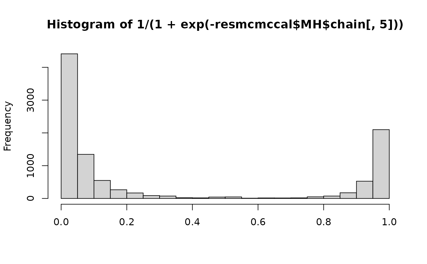

plot(1/(1+exp(-resmcmccal$MH$chain[,5])),type="l",ylab=expression(theta))

plot(1/(1+exp(-resmcmccal$MH$chain[,1])),type="l",ylab=expression(rho[1]))

plot(1/(1+exp(-resmcmccal$MH$chain[,2])),type="l",ylab=expression(rho[2]))

plot(1/(1+exp(-resmcmccal$MH$chain[,5])),1/(1+exp(-resmcmccal$MH$chain[,1])),ylab=expression(rho[1]),xlab=expression(theta))

plot(1/(1+exp(-resmcmccal$MH$chain[,5])),1/(1+exp(-resmcmccal$MH$chain[,2])),ylab=expression(rho[2]),xlab=expression(theta))

plot(resmcmccal$MH$chain[,5],resmcmccal$MH$vlogpost,main="posterior distribution with respect to theta")

Two-step discrepancy screening

We estimate the parameter \(\theta\) by the median of the posterior distribution

thetamed = median(1/(1+exp(-resmcmccal$MH$chain[,5])))

We regenerated the residuals for the calibrated value of \(\theta\)

print(thetamed)
#> [1] 0.06779808
modthetamed <- simulator(x, thetamed)
Rexp <- (y-modthetamed) 
resmcmcthetamed <- (MCMC(nMWG,nMet,parwalkinit,init,Rexp,tdistFULL,1.9,parprior,TRUE,calibration1))

We have a look a the posterior samples of \((\rho_1,\rho_2)\)

#resmcmcthetamed$MH$AccepRate
plot(1/(1+exp(-resmcmcthetamed$MH$chain[,1])),type="l",ylab=expression(rho[1]))

plot(1/(1+exp(-resmcmcthetamed$MH$chain[,2])),type="l",ylab=expression(rho[2]))

We estimate the parameter \(\theta\) by the mean of the posterior distribution

thetamean = mean(1/(1+exp(-resmcmccal$MH$chain[,5])))

We regenerated the residuals for the calibrated value of \(\theta\)

print(thetamean)
#> [1] 0.3266593
modthetamean <- simulator(x, thetamean)
Rexp <- (y-modthetamean) 
resmcmcthetamean <- (MCMC(nMWG,nMet,parwalkinit,init,Rexp,tdistFULL,1.9,parprior,TRUE,calibration1))

We have a look a the posterior samples of \((\rho_1,\rho_2)\)

resmcmcthetamean$MH$AccepRate
#> [1] 0.4652
plot(1/(1+exp(-resmcmcthetamean$MH$chain[,1])),type="l")

plot(1/(1+exp(-resmcmcthetamean$MH$chain[,2])),type="l")

For both cases, we compute the probabilities of activness:

computeProbActive(resmcmcthetamed$MH$chain[thinning,1:pgamma])
#> [1] 0.66831376 0.01308459
computeProbActive(resmcmcthetamean$MH$chain[thinning,1:pgamma])
#> [1] 0.16860320 0.03094512

Repetitions

We repeat the data generation and the computation of probabilities of activeness over \(100\) replications :

We load and format the results:

load("../inst/simuCalibOrNot.Rdata")

lPROBAS=lapply(1:length(RESlist),function(k){
  out = RESlist[[k]]$probaActive
  out
})

PROBAS=as.data.frame(do.call(rbind,lPROBAS))
names(PROBAS) = c("nominal","calibration","median","mean")
PROBAS$variable=rep(c(1,2),100)
PROBAS$sim=rep(1:100,each=2)

library(reshape2)
dfProb = melt(PROBAS,id.vars = c("variable","sim"))
#head(dfProb)
names(dfProb)[3:4]=c("type","prob")
dfProb$variable=factor(dfProb$variable)

We plot the probabilities of activness in all cases

library(ggplot2)
ggplot(dfProb,aes(x=type,y=prob,col=variable))+geom_boxplot()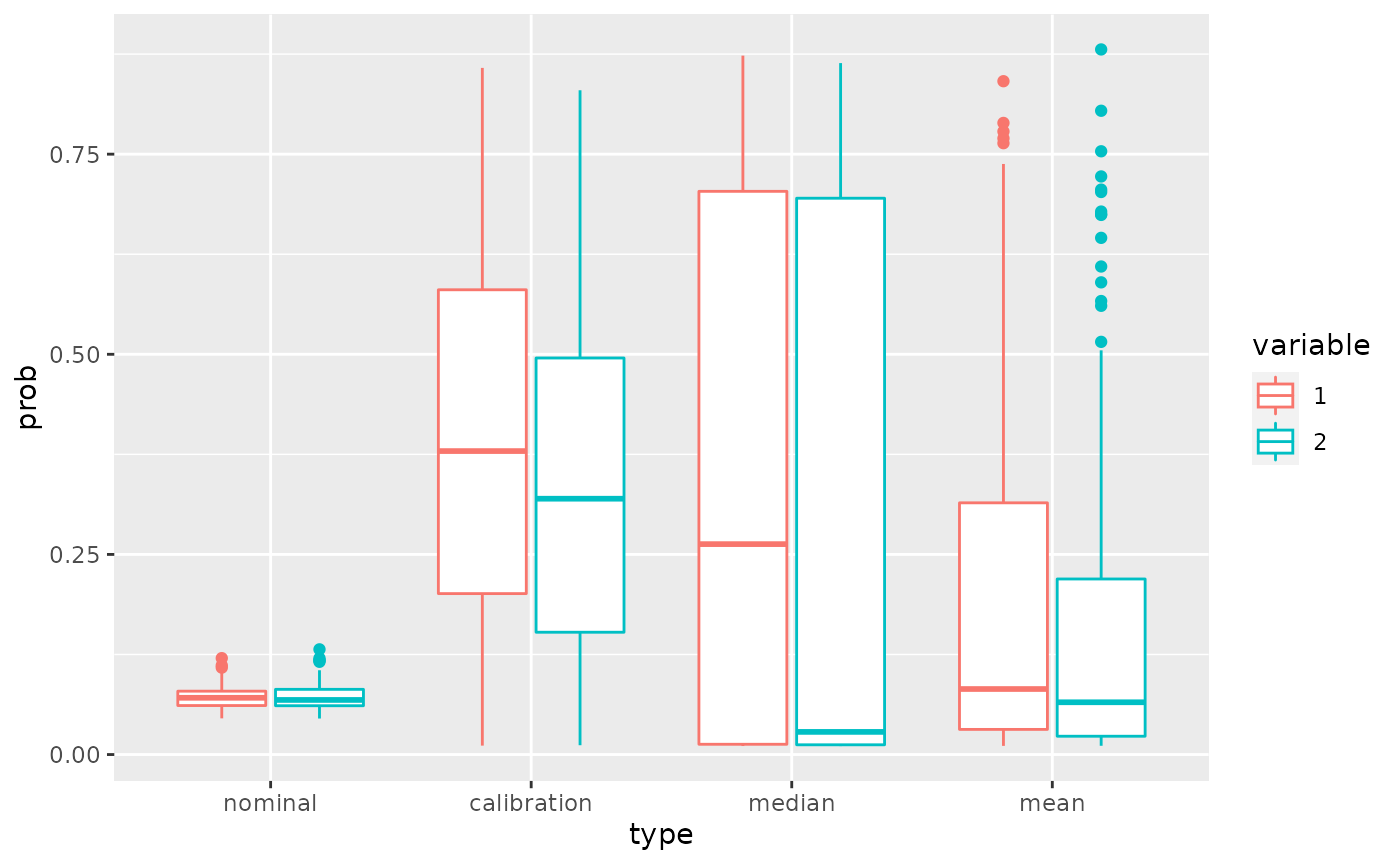

ggplot(dfProb,aes(x=sim,y=prob,col=variable,shape=type,linetype=type))+geom_point()+geom_line()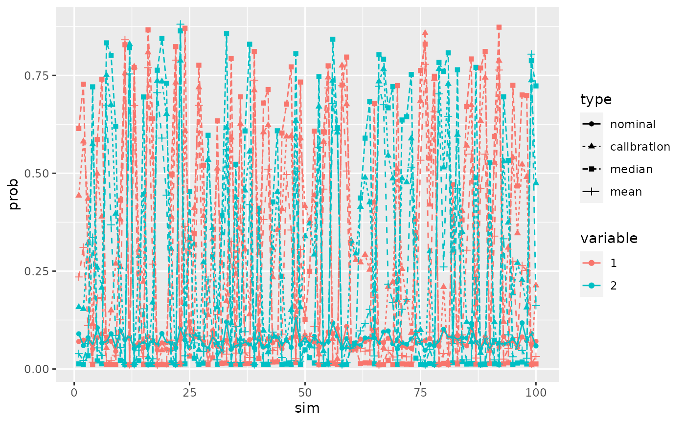

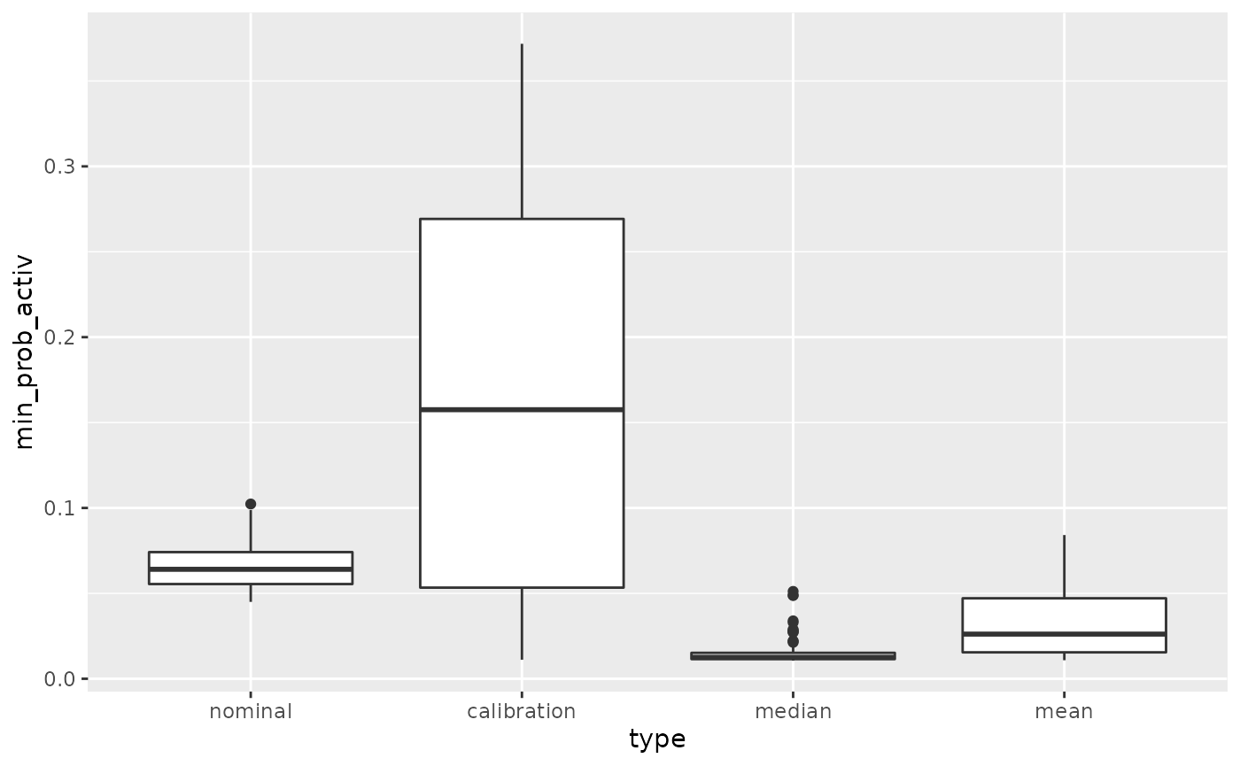
The main interest is that with the calibration method the probability of activeness is never too small for both variables

# min des 2
lPROBAS=lapply(1:length(RESlist),function(k){
  out = RESlist[[k]]$probaActive
  apply(out,2,min)
})


PROBAS=as.data.frame(do.call(rbind,lPROBAS))
names(PROBAS) = c("nominal","calibration","median","mean")
dfProb = melt(PROBAS)
#> No id variables; using all as measure variables
head(dfProb)
#>   variable      value
#> 1  nominal 0.07009146
#> 2  nominal 0.05970586
#> 3  nominal 0.07721193
#> 4  nominal 0.05130185
#> 5  nominal 0.07994864
#> 6  nominal 0.06635595
names(dfProb)[1:2]=c("type","min_prob_activ")

ggplot(dfProb,aes(x=type,y=min_prob_activ))+geom_boxplot()