ExampleScenario
ExampleScenario.Rmd
library(PIPScreening)Scenario setting
True physical model is \[\zeta_i(x_1,\ldots,x_5)=\frac{|4 x_{1}^2 -2| + \theta_1}{1+\theta_1} +\frac{|4 x_{3} -2| + \theta_3}{1+\theta_3}\,.\]
The field data are for \(i=1,\ldots,N\) : \[y_i=\zeta(\mathbf{x_i})+\epsilon_i\,.\]
where \(\epsilon_i\overset{iid}{\sim}\mathcal{N}(0,\sigma^2_\epsilon)\).
Our computer model / simulator is \[f(\mathbf{x},\boldsymbol{\theta})= \frac{|4 x_{1} -2| + \theta_1}{1+\theta_1} +\frac{|4 x_{2} -2| + \theta_2}{1+\theta_2} +\frac{|4 x_{3} -2| + \theta_3}{1+\theta_3}\,.\] Thus, \(x_1\) is incorrectly taken into account in \(f\) and \(x_2\) is taken into account while it has no effect in the “real” physical system. The parameter \(\boldsymbol{\theta}\) is a model parameter, it may be fixed or be to calibrate.
Data simulation
Field data:
N<-50
beta<-c(1,0,1,0,0) # binary vectors indicating which input variables x are used in the physical simulator (1) or not (0)
theta<-4:8/10 # choice of the theta (here same size as x)
sd<-0.05
p <- c(2,1,1,1,1) # power for the x's
x1 <- runif(N,0,1)
x2 <- runif(N,0,1)
x3 <- runif(N,0,1)
x4 <- runif(N,0,1)
x5 <- x3 + rnorm(N,sd=.2)
covargal <- cbind(x1^p[1],x2^p[2],x3^p[3],x4^p[4],x5^p[5])
mu <- simGal(covargal,theta,beta) # physical system
y <- mu + rnorm(N,0,sd) # field exp by adding noise
Preparing the data for running the MCMC run:
x <- cbind(x1,x2,x3,x4,x5)
covarmod <- cbind(x1,x2,x3) # model covariates
mod <- sim3(x, theta[1:3]) # output of computer model
xnorm <- (x - matrix(apply(x,2,min),nrow=nrow(x),ncol=ncol(x),byrow=T))/matrix(apply(x,2,max)-apply(x,2,min),nrow=nrow(x),ncol=ncol(x),byrow=T) # normalization
Yexp <- y; Xexpnorm <- xnorm; Xexp <- x;  Rexp <- (y-mod)
Posterior sampling with or without calibration
Without calibration (\(\boldsymbol{\theta}\) being fixed to its true value)
calibration1 <- list(computermodel=sim3,Yexp=Yexp,Xexp=Xexp,FALSE)
tdistFULL <- tensordist(xnorm)
pgamma <-  5
parwalkinit  <-  c(rep(.1,pgamma),.1,.1)
init  <-  c(rep(0,pgamma),.004,.2)
a <- TRUE
cpt <- 0
parprior <- rbind(matrix(1,nrow=pgamma,ncol=2),c(4,.02),c(3,1))
nMWG <- 2000
nMet <- 2000
resmcmc <- (MCMC(nMWG,nMet,parwalkinit,init,Rexp,tdistFULL,1.9,parprior,TRUE,calibration1))
ptheta <- 3
With calibration, we just changed some options to run this version such as the calibration2 list which indicates that calibration should be done, the init2 vector which gives the initial value for all the parameters (now it includes the \(\theta\)s) and the parwalkinit2 which gives the parameter for the random walk.
calibration2 <- list(computermodel=sim3,Yexp=Yexp,Xexp=Xexp,TRUE)
parwalkinit2 <- c(rep(.1,pgamma),.1,.1,rep(.1,ptheta))
init2 <- c(rep(0,pgamma),.004,.2,rep(.5,ptheta))
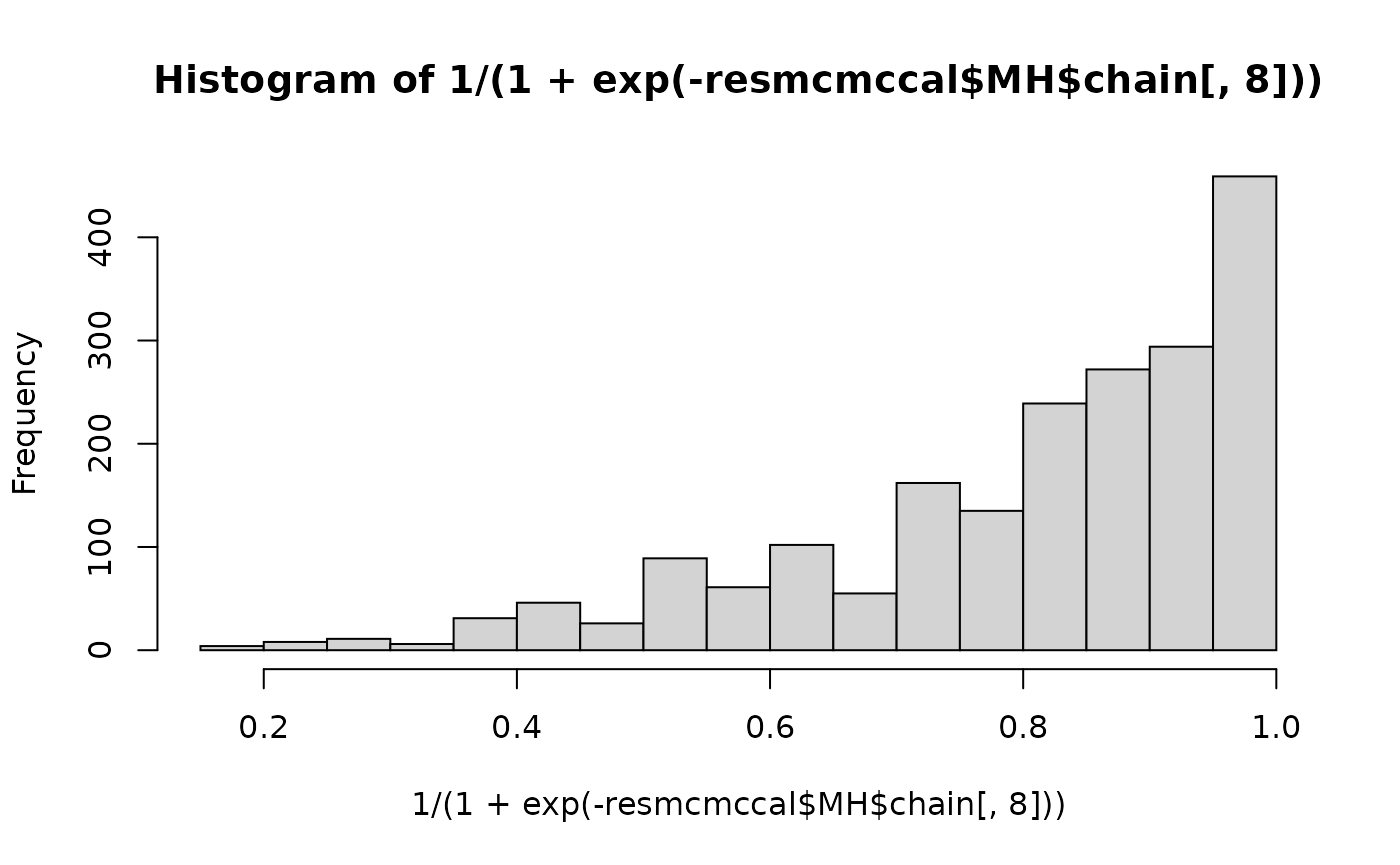
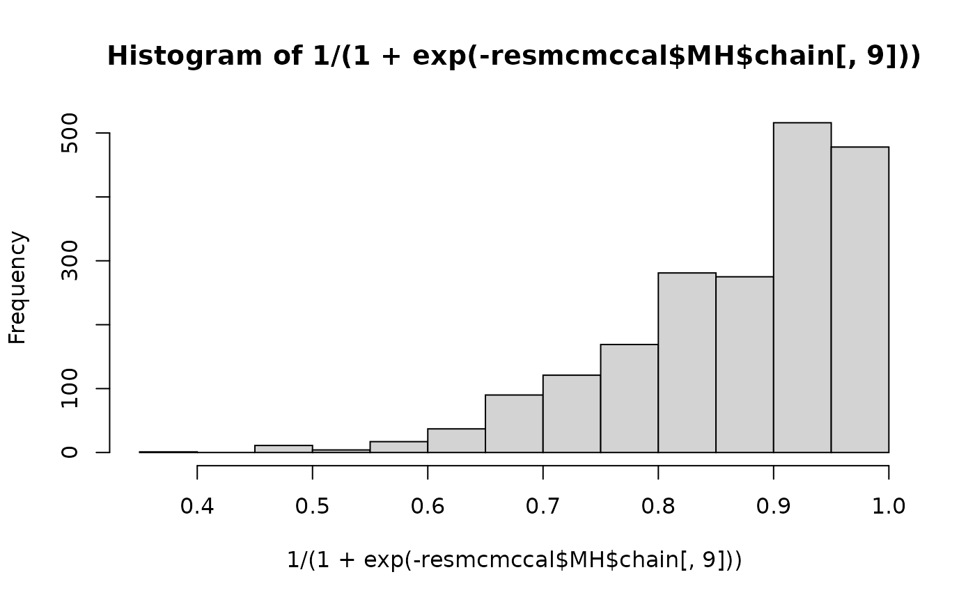
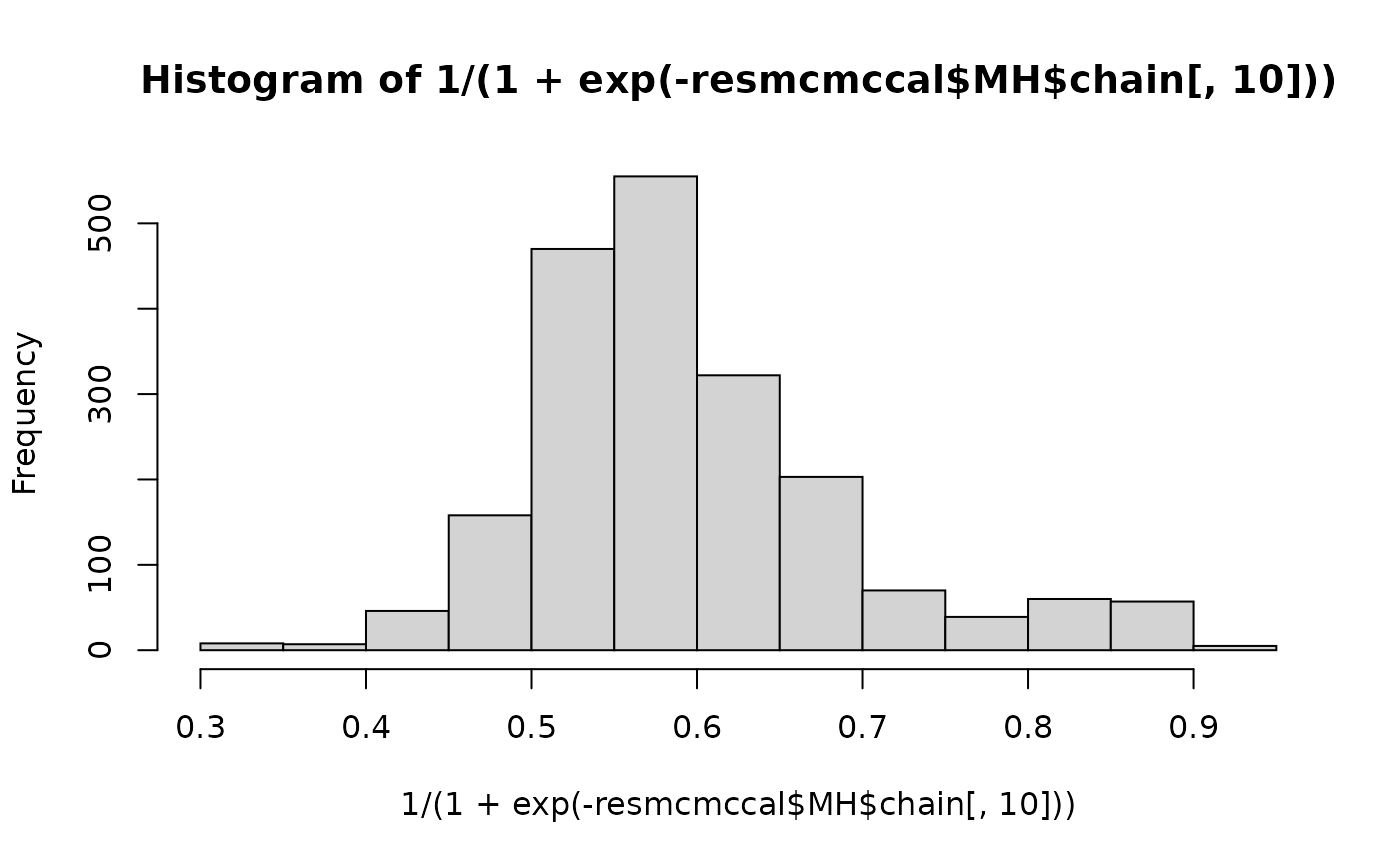
resmcmccal <- MCMC(nMWG,nMet,parwalkinit2,init2,Rexp,tdistFULL,1.9,parprior,TRUE,calibration2)The sampling is done with a Metropolis within Gibbs algorithm and then with a Metropolis algorithm. From the MwG algorithm, a covariance matrix is derived for the random walk in the upcoming Metropolis algorithm. Some adaptations are performed to set the exploration step. Note the number of iterations are really low in this vignette to limit its compilation time.
Computation of probabilites of activeness
First computed from the posterior sampling without calibration and then computed from the posterior sampling which deals with calibration. We obtain then two vectors of probabilities which give for each variable the probability that a variable is active in the discrepancy. Here we expect that the fist variable (because of the power 2 in the physical system) and the second variable (because of the mismatch between the physical system and the computer model) to be active.
computeProbActive(resmcmc$MH$chain[,1:pgamma])
#> [1] 1.00000000 0.99999961 0.01459635 0.01206288 0.01590240
computeProbActive(resmcmccal$MH$chain[,1:pgamma])
#> [1] 1.00000000 0.99999610 0.01302021 0.01179403 0.01574140